2021

Dose assessment methods used to evaluate the radiation exposures
from nuclear testing in the atmosphere, with emphasis
on the tests conducted in French Polynesia

Types and characteristics of dose assessment

Information on average doses to large groups of people

Many radiation measurements were made throughout the world during the period of atmospheric testing. These radiation measurements were essentially made to verify that the populations were not submitted to excessive levels of exposure. The United Nations Scientific Committee on the Effects of Atomic Radiation (UNSCEAR) was established in 1955 to compile and assemble the national reports and to evaluate them. UNSCEAR published its reviews of radioactive fallout and resulting doses from atmospheric nuclear weapons tests within a few years’ intervals from 1958 until 2000 (UNSCEAR, 1958, 1962, 1966, 1969, 1972, 1977, 1982, 1993, 2000). The principal aims of the UNSCEAR reports was to estimate the average deposition densities of the most important radionuclides according to 10^o latitude bands and the population-weighted doses over the entire populations of the northern and southern hemispheres, and of the entire world. As shown in Figure 1, the radioactive cloud produced by the explosion can be widely dispersed at the continental scale within a few days. The part of the radioactive cloud that is contained in the troposphere will circle the world, roughly in the same latitude band, in 20 to 30 days, while the part of the radioactive cloud that reaches the stratosphere will remain there during a year or two before descending to the ground.

Figure 1 Dispersion of the radioactive cloud produced by an atmospheric nuclear weapons test

Figure 1

Figure 1 Dispersion of the radioactive cloud produced by an atmospheric nuclear weapons test

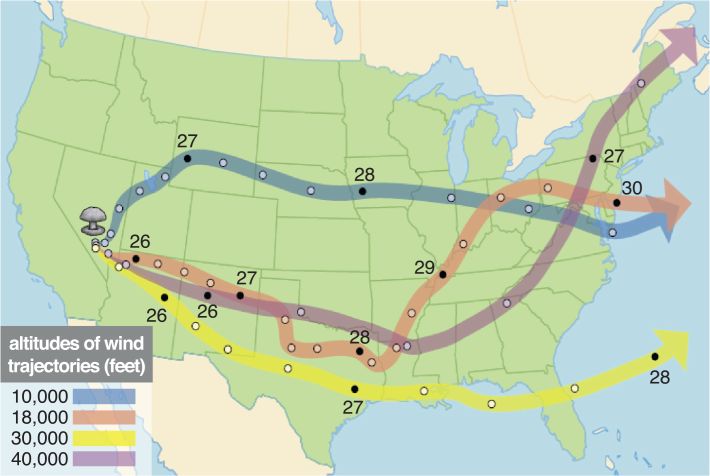UNSCEAR is mainly concerned with the collective effective dose commitment for the world population. An example of results presented in UNSCEAR Reports is shown on Table 1. A summary of the temporal variation of the doses can be found in (Bouville et al., 2002).

Tableau 1 Collective effective dose to the world population committed from atmospheric nuclear testing (based on UNSCEAR, 1993)

Estimation of doses to critical groups

A range of human exposure pathways is possible as a result of an atmospheric nuclear weapons test (see Figure 2). The radiation measurements carried out in the local area (which typically extends to 200-300 km from the site of the explosion) are in part used to make sure that local populations were not subjected to excessive levels of radiation or that the maximally exposed critical groups received doses below the regulatory limits. These dose assessments are carried out using conservative assumptions and are not, as a rule, available in the open literature, although there are exceptions (see, for example, Ministère de la Défense, 2006 and Royal Commission into British Nuclear Tests in Australia, 1985). A review of the available information on the radiation doses to local populations near nuclear weapons test sites worldwide was published by Simon and Bouville (2002).

Input data for use in epidemiologic studies of risk projection

Beginning in the late 1970s, a push was made by the U.S. Government to obtain more detailed and realistic information on the radiation doses received by the populations residing in the proximity of the Nevada Test Site (NTS). In 1979, the U.S. Department of Energy established the Off-site Radiation Exposure Review Project (ORERP) to: (1) collect and organize at a central location all relevant documents and data pertaining to fallout in the off-site area and make these documents available to the public, and (2) produce a dosimetric re-evaluation of the off-site area characterized by region, community/locale, and age/occupation (Church et al., 1990). The methodology of dose assessment that was developed by ORERP (Anspaugh and Church, 1986; Hicks, 1982; Whicker and Kirchner, 1987), as well as the data that were collected and processed, form the basis upon which the epidemiologic studies on fallout from nuclear weapons studies conducted in the U.S., either completed or ongoing, relies upon. In the area of risk projection, these studies, which were mandated by the U.S. Congress, include: (1) a National Cancer Institute (NCI) study of thyroid doses from ¹³¹I intakes, and resulting thyroid cancer, received by populations across the continental USA (NCI, 1997), (2) a study jointly conducted by Centers for Disease Control and Prevention (CDC) and NCI on the feasibility to reliably estimate the health consequences to the American population from nuclear weapons tests conducted by the U.S. and other nations (DHHS, 2005), (3) a study of radiation doses and cancer risks in the Marshall Islands from U.S. nuclear weapons tests (Simon et al., 2010a), and (4) a study to estimate radiation doses and cancer risks from radioactive fallout from the Trinity nuclear test (NCI, 2008). The doses calculated in these studies are as unbiased as possible and are for representative individuals with typical dietary, residential, and lifestyle habits. The dose values are then applied to the population groups corresponding to the representative individuals. An example of results obtained in this manner is shown in Table 2.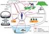

Figure 2 Illustration of pathways of human exposure resulting from an atmospheric nuclear weapons test

Figure 2

Figure 2 Illustration of pathways of human exposure resulting from an atmospheric nuclear weapons test

Tableau 2 Best estimates of cumulative acute internal and chronic internal doses (mGy) for four organs and of external dose (at all organs) to adults of four representative population groups (based on Simon et al., 2010a)

^a RBM: Red bone marrow.

Input data for use in analytical epidemiologic studies

The ORERP methodology and data were also used in the framework of analytical epidemiologic studies (case-control or cohort), in which individual doses to all study subjects need to be estimated: (1) the Utah leukemia case-control study, related to radiation exposures resulting from NTS atmospheric tests (Simon et al., 1995), (2) the Utah thyroid cohort study, also related to the NTS tests (Till et al., 1995), (3) the Semipalatinsk cohort study, conducted jointly by U.S. and Russian investigators (Gordeev et al., 2006 a and b), and (4) the French Polynesia thyroid case-control study (Drozdovitch et al., 2008, 2019, 2020a, 2020b). In the analytical epidemiologic studies, information, as complete and reliable as possible, needs to be obtained on the residential, dietary, and lifestyle habits of all study subjects, generally through the use of a combination of individual interviews, focus groups, and available records. Because the individual dose estimates for analytical epidemiologic studies must be as unbiased as possible, it is necessary to use as many radiation measurements (exposure rates, radionuclide concentrations in air, water, foodstuffs, etc.) as possible. Fortunately, as will be seen later, large numbers of such measurements were made in French Polynesia at the time of the atmospheric tests (Coulon et al., 2009).

An example of dosimetry results obtained in an analytical epidemiologic study is shown in Table 3.

Tableau 3 Summary of active marrow doses (mGy) for the 6507 study subjects of the Utah leukemia case-control study (based on Simon et al., 1995)

Validation of the dose estimates

The ideal approach is to estimate the dose for a suitable proportion of the targeted subjects using a biologically-related measure that correlates highly with dose and to compare the measurements made by the primary approach with estimates of doses made by other means. There are biodosimetric techniques, notably fluorescence in situ hybridization (FISH) and electron paramagnetic resonance (EPR), for validation of the external doses. The EPR technique was used to validate the external doses related to the tests conducted at Semipalatinsk (Sholom et al., 2007), but it does not seem to have been applied to any other fallout study related to nuclear weapons tests. In the NTS study conducted by NCI (1997), the ¹³¹I concentrations measured in urine were used to indirectly validate the thyroid doses.

Uncertainties in the dose estimates

A single ideal approach to evaluate and account for all dosimetric uncertainties is not available but is an area of active research (NCRP, 2009). Until recent years, the evaluation of the uncertainties consisted of numerical simulations in which variability and lack-of-knowledge uncertainties were combined in Monte-Carlo simulations. In that method, probability density distributions are assigned to the parameter values that are deemed to have a substantial influence on the dose estimate and multiple realizations of individual doses are estimated (NCRP, 1996). The primary limitation of many such simulations is that shared errors and intra-individual correlations are not accounted for. A more sophisticated method, the two-dimensional Monte-Carlo procedure, was used in the Semipalatinsk study to separate and distinguish between the shared and the unshared components (Land et al., 2015; Simon et al., 2015). In most studies, uncertainties were evaluated in a subjective manner, if at all.

Methods of dose assessment used for the U.S. and Russian tests

Estimation of external doses

Estimation of the normalized outdoor exposure rates

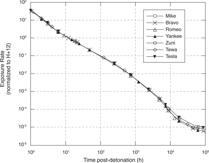
The temporal variation of the exposure rate cannot be represented by a simple equation that is valid at all times, but it can be approximated as t^-1.2 for times between 30 minutes to 200 days after the explosion (Glasstone and Dolan, 1977). This is the equation that was typically used for the dose assessments related to the Russian tests (Gordeev et al., 2006a). In the United States, the temporal variation of the exposure rates was established for all important tests as a 10-component multi-exponential function, which is rather complex but can be applied to any time after the explosion. For a given degree of fractionation between refractory and volatile radionuclides (R/V fractionation ratio), there is little variation from one test to another (see Figure 3).

Estimation of the total exposure

The total exposure is calculated as the product of the outdoor exposure rate at H + 12 h and of the integral over time of the normalized outdoor exposure rate, shown in Figure 3, taking the fractionation ratio R/V into account. The fractionation ratio reflects the fact that particles of all sizes are in the radioactive cloud. The large particles, with sizes > 50 μm, are enriched with refractory radionuclides, whereas the small particles, with sizes < 50 μm, are enriched with volatile radionuclides. Because the large particles deposit more quickly than the small particles, meaning that they reach the ground at smaller distances from the site of the explosion, the value of R/V decreases as the distance from the site of the explosion increases. The value of R/V, which usually is in the range from 0.5 to 3.0, is estimated to vary as a function of TOA/T_cr, where the critical time T_cr is the length of time since detonation for all particles > 50 μm to be deposited (Beck et al., 2010). For locations where TOA > T_cr, all deposited particles are smaller than 50 μm and R/V = 0.5.

Figure 3 Variation of the exposure rate with time for several atmospheric tests for a fractionation ratio (R/V) of 0.5 (Bouville et al., 2010)

Figure 3

Figure 3 Variation of the exposure rate with time for several atmospheric tests for a fractionation ratio (R/V) of 0.5 (Bouville et al., 2010)

In the calculation of the total exposure, the lower bound is TOA and the upper bound is the time until which the dose is to be calculated, usually 1 or 50 years. The exposure rate is usually expressed in mR h^-1 and the total exposure in Roentgen (R). Because most radionuclides produced by a nuclear test have very short half-lives, the exposure rate decreases rapidly with time (see Figure 3), so that almost the totality of the exposure is obtained during the first year after the detonation.

Estimation of the organ and tissue doses

In order to calculate the organ and tissue dose from the outdoor exposure values, one must first convert exposure to dose in air using a factor of 8.75 10^-3 Gy R^-1. Then, a factor of 0.75 Gy Gy^-1 is typically used to convert from dose in air to dose in tissue or organ of an adult (UNSCEAR, 1993). This factor varies with the energy of the gamma ray and with the orientation with respect to radiation incidence, as well as with the organ or tissue that is considered and with the anthropomorphic characteristics of the person. Because there is little difference between the values of the conversion factor from an organ to another for gamma rays of a few hundred keV that are typical for fission products, the same value can be used for adults for all organs and tissues usually considered in fallout studies. However, calculations using anthropomorphic phantoms of different ages indicate that slightly higher values are obtained for younger ages (Jacob et al., 1990). Based on those calculations, the conversion factors for younger (< 3 y, including in utero) and older (3 through 14 y) children were derived in the Marshall Islands study by multiplying the adult conversion factors by 1.3 and 1.2, respectively (Bouville et al., 2010). Finally, the calculation of the outdoor dose must take the fraction of time spent outdoors into account. If it is assumed to be 0.2 (UNSCEAR, 1993), the overall conversion factor from outdoor exposure to tissue dose is 8.75 10^-3 (Gy R^-1) × 0.75 (Gy Gy^-1) × 0.2 = 1.3 10^-3 Gy R^-1 for representative adults. For specific individuals, the value of the fraction of time spent out of doors must be obtained from individual interviews or derived from focus groups or interviews of experts.

The calculation of the external tissue dose received indoors due to exposure outdoors is carried out in a similar manner, the only differences being that the fraction of time spent being exposed is different (1 – 0.2 = 0.8 for the example given above) and that the shielding provided by the building structure must be taken into account. If the shielding factor is assumed to be 0.2 (UNSCEAR, 1993), the overall conversion factor from indoor exposure to tissue dose is 8.75×10^-3 (Gy R^-1) × 0.75 (Gy Gy^-1) × 0.8 × 0.2 = 1.05×10^-3 Gy R^-1 for representative adults. For specific individuals, the value of the fraction of time spent indoors must be obtained from individual interviews or derived from focus groups or interviews of experts; the value of the shielding factor is ideally obtained from measurements. In the absence of measurements, literature values (for example, Glasstone and Dolan, 1977) are used.

Estimation of internal doses

Internal doses from nuclear weapons tests are essentially due to inhalation of contaminated air and ingestion of contaminated water and foodstuffs. The method used to estimate the internal doses depends on the environmental and human radiation data that are available. The bioassay measurements performed on exposed persons are the data of choice: they are the foundation of the dose estimates for the Marshall Islands study (Simon et al., 2010b), as the doses from acute intakes of radionuclides are derived from historical measurements of ¹³¹I in pooled samples of urine collected from adults about 2 weeks after the Bravo test (Harris et al., 2010) and the doses from intakes of long-lived radionuclides are based on measurements of whole-body activity of ¹³⁷Cs, ⁶⁰Co, and ⁶⁵Zn (Lessard et al., 1984). For the other U.S. tests and for the Russian tests, bioassay data are either non-existent or limited to a small of persons (see, for example NCI, 1997). This is true as well for environmental radiation data. In most cases, the assessment of internal doses related to U.S. and Russian tests is based on models of environmental transfer from the activity deposited on the ground to the radionuclide concentrations in air, water, and foodstuffs; it generally consists of 5 steps: (1) estimation of the ground deposition densities (Bq m^-2), (2) estimation of radionuclide concentrations in the vegetation and in soil (Bq kg^-1), (3) estimation of radionuclide concentrations in air (Bq m^-3), water (Bq L^-1), milk (Bq L^-1), plants, animals and animal products (Bq kg^-1), (4) estimation of internal doses from inhalation (Gy), and (5) estimation of internal doses from ingestion (Gy).

Estimation of the ground deposition densities of each radionuclide

The data reported by Hicks (1981) provide not only the variation of the exposure rate with time after the detonation for values of R/V of 1.0 and 0.5, but also the corresponding ground deposition densities of a large range of radionuclides. Beck et al. (2010) extended these calculations to other values of R/V appropriate to fallout near the site of the explosion.

Estimation of vegetation and soil radionuclide concentrations

where M is the maximum interception (unitless), α is the foliar interception constant (m² kg^-1 (dry mass)), and Y is the standing crop biomass (kg (dry mass) m^-2). The values of Y may vary according to the ecozone and the type of vegetation, while the values of α and M may vary according to the type of vegetation (Thiessen and Hoffman, 2018).

Estimation of radionuclide concentrations in air, water, and foodstuffs

The estimation of radionuclide concentrations in air (Bq m^-3), water (Bq L^-1), milk (Bq L^-1), plants, animals and animal products (Bq kg^-1) is conducted using a range of models well described in the literature (e.g., NCI, 1997; Thiessen and Hoffman, 2018; Whicker and Kirchner, 1987).

Estimation of internal doses from inhalation

For example, in a NTS study, the relationship between the deposited activity on the ground, A_gd, of radionuclide Z at location L, and the time-integrated concentration of the respirable-sized particles in air during the passage of the radioactive cloud, IC_{air, cloud}, was estimated by Simon et al. (1990) to be:

The inhalation dose due to resuspension has not been included in any U.S. or Russian study, but there are plans to include it in the Trinity study (NCI, 2007). The calculation of the time-integrated concentrations in air due to resuspension IC_air,res(Z,L) in Bq d m^-3, would be derived from measured values of the resuspension factor S_f(t), which is the ratio of the air concentration and of the deposited activity (Anspaugh et al., 2002; Maxwell and Anspaugh, 2011):

Figure

Estimation of internal doses from ingestion

The internal doses (age-dependent organ-specific doses) from ingestion are derived from the estimated time-integrated radionuclide concentrations in water and foodstuffs, taking into consideration the commercial distribution of the considered foodstuffs, the consumption rates of the study subjects, the reduction in activity due to processing and culinary factors, and the dose coefficients from ingestion intake to absorbed doses in the organs and tissues under consideration (NCI, 1997; Ng et al., 1990). For specific individuals, the food consumption rates of the study subjects must be obtained from individual interviews or derived from focus groups or interviews of experts (Schwerin et al., 2010; Drozdovitch et al., 2011).

Methods used for the tests conducted in French Polynesia

France conducted forty-one atmospheric nuclear weapons tests (and five safety tests) in French Polynesia in 1966-1974 (UNSCEAR, 2000; Bataille and Revol, 2002). The nuclear test sites were two atolls, Muruora and Fangataufa, located in the southeastern part of Tuamotu-Gambier archipelago at about 1150 km from Tahiti, the most populated island in French Polynesia.

The network of environmental surveillance included different islands representative of the five French Polynesian archipelagoes. In selecting these islands, environmental and ecological diversity, heterogeneous demography, and predominant winds that potentially affected the consequences of nuclear tests were taken into account. Radiological monitoring on land was supplemented with measurements on buoys, ships, and aircraft (Coulon et al., 2009; IAEA, 2009-2010). In addition, 25 campaigns of anthropogammametry measurements were conducted among the populations of the islands close to the nuclear sites; unfortunately, the results, expressed in terms of triage index, cannot be used for dose assessment purposes as no additional information is available.

The methodologies used by the French authorities (Ministère de la Défense, 2006; DSND, 2006a, 2006b) and by Inserm in a study of thyroid cancer in French Polynesia (Drozdovitch et al., 2008, 2019, 2020a, 2020b) are presented in turn.

Dose assessment by the French authorities

The French authorities reported doses, in terms of effective doses and of thyroid doses, for the most important tests and for two age categories (1-2 year old and adults) in the most exposed populations (Ministère de la Défense, 2006). The main purpose of the dose assessments was to make sure that the dose levels were below the regulatory limits.

Assessment of the external doses

• Immersion dose during the passage of the radioactive cloud

The method used by the French authorities to calculate the immersion doses was based on the measured global β activity of the ground deposition density, expressed in Bq m^-2. The activity of each of the approximately 70 radionuclides contributing substantially to the global β activity, as well as their variation with time after detonation, were derived from the JEFF database2

JEFF: Joint Evaluated Fission and Fusion nuclear data library (Nuclear Energy Agency).

(AEN, 2005). The time-integrated concentration in air, expressed in Bq s m^-3, was then obtained using a deposition velocity, the value of which varied according to estimated TOA at the location considered and the occurrence, or not, of rain. Deposition velocities ranging from 10^-3 to 10^-1 m s^-1 were used for TOAs shorter than one day. The final step of the calculation of the immersion dose consisted in applying an appropriate effective dose coefficient, expressed in Sv per Bq s m^-3, to each radionuclide (Eckerman and Ryman, 1993) and in summing the results over the 70 radionuclides. The reduction of the dose due to shielding while indoors was taken into account, using a protection factor of 0.5 if the radioactive cloud arrived during the night or while the population was sheltered. The dependence of the dose with age was not taken into account.

• External dose resulting from ground deposition of fallout

In the method used by the French authorities, the ground deposition density of each of the approximately 70 radionuclides contributing substantially to the external dose is calculated in the same manner as is done in the calculation of the immersion dose. The effective dose rate, expressed in Sv h^-1, for each radionuclide is then calculated using an appropriate effective dose rate coefficient (Eckerman and Ryman, 1993). Integrating over the time of exposure, taking radioactive decay into account, yields the external effective dose due to the radionuclide under consideration. Summation over the approximately 70 radionuclides leads to the total external effective dose due to the ground deposited activity. Modifying factors were applied to this result: (1) a reduction factor of 2/3 based on the assumption that people spent part of their time in the contaminated area, and (2) when the radioactive cloud arrived during the night, it was assumed that the populations, being indoors, were not exposed during the first 6 hours after TOA.

It is worth noting that, although exposure rates were measured at various locations after each test, the measured values do not appear to have been preferentially used in the calculation of the external doses by the French authorities, which used the measured global β activity of the ground deposition density as the starting point of the dose calculation. This is in sharp contrast with the method used in the U.S. studies, in which the ground deposition density did not have to be measured in order to calculate the external dose, although it should be recognized that if the measurements of the outdoor exposure rates were missing or insufficient, the exposure rates were derived from the ground deposited activity, measured for example using gummed film (Beck et al., 1990; Bouville and Beck, 2000).

• Internal dose resulting from inhalation of radioactive materials

• Internal dose resulting from ingestion of water, milk, and foodstuffs

The consumption rates of the foodstuffs for representative adults of the five archipelagoes of French Polynesia were established on the basis of dietary surveys conducted in 1965 and 1985 (Lederman, 1965; Grouzelle et al., 1985). Only locally produced foodstuffs were considered. The consumption rates of children were derived from the consumption rates of adults.

The effective dose coefficients and the thyroid dose coefficients were taken from ICRP publications (ICRP, 1995, 1996a, 1996b).

• Dose estimates

Radioactive fallout from the atmospheric tests conducted in French Polynesia was extremely small when the actual meteorological conditions were consistent with those that were predicted. However, this was not the case for several tests (including Aldebaran (2 July 1966), Rigel (24 September 1966), Arcturus (2 July 1967), Encelade (12 June 1971), Phoebé (8 August 1971), and Centaure (17 July 1974)). Relatively important fallout from those tests occurred either on Tureia (the closest atoll to the test sites, located at about 110 km), the Gambier Islands (450 km from the test sites), or Tahiti (including Pirae, Hitiaa, and Taravao), located 1150 km away from the test sites. The estimates of the thyroid doses for 1-2 y old children (mGy) and of the effective doses (mSv) for adults are presented in Tables 4 and 5 at the most exposed locations for each of the exposure pathways taken into consideration.

Tables 4 and 5 show that the consumption of water and seafood were important exposure pathways in the atolls and islands close to the test sites, where the populations were small and the diet was limited to a few staples. In Tahiti, where more than half of the total French Polynesian population resided, there was a large variety of food products, including cow’s milk, and the consumption of water played a relatively minor role.

Tableau 4 Estimated thyroid doses to 1-2 y old children (mGy), calculated by the French authorities for the 6 tests with significant fallout (based on Ministère de la Défense, 2006)

Tableau 5 Estimated effective doses to adults (mSv), calculated by the French authorities for the 6 tests with significant fallout (based on Ministère de la Défense, 2006)

Dose assessment for the Inserm study of thyroid cancer
in French Polynesia

To evaluate the potential role of atmospheric nuclear weapons testing on a high incidence of thyroid cancer observed since 1985 in French Polynesia (de Vathaire et al., 2000), a population-based case-control study of thyroid cancer was performed. The study consisted of two phases. Phase I included all alive cases of thyroid cancer developed between 1985 and 2003 in persons who were children, adolescents, and young adults at the time of atmospheric nuclear testing. Epidemiological aspects of Phase I and estimates of risk of thyroid cancer were published by de Vathaire et al. (2010). Overall, 602 subjects, both cases and controls, were included in the risk analysis, which was performed using thyroid doses calculated in 2008 by means of the “Thyroid Dosimetry 2008 system” (TD08) (Drozdovitch et al., 2008). In 2014-2017, Inserm undertook Phase II of the epidemiological study, including 348 additional subjects, thus resulting in a total of 950 subjects. Because of deficiencies in TD08, mainly related to limitations in the input data, the dosimetry system was improved for the assessment of thyroid doses for all subjects of the epidemiologic study. Unit 605 of Inserm (currently Unit 1018) coordinated the case-control study.

The methodology of the dose assessment and the dose estimates for Phase I of the study were published by Drozdovitch et al. (2008). The radiation dose to the thyroid gland had to be evaluated for each study subject. However, the following limitations of TD08 were recognized:

• One of the major deficiencies was the limited information on lifestyle in French Polynesia in the 1960s-1970s that was available for TD08. Individual data for each study subject had been collected by means of personal interviews on (i) places of residence in 1966-1974; (ii) consumption rates of various foodstuffs at age 15; (iii) source of drinking water, i.e. individual cistern, communal cistern, other; and (iv) type of residence, i.e. apartment or house. However, important information, needed for precise dose estimation, was missing in the questionnaire; this included: (i) the type of construction materials used to build the residences; (ii) the time spent indoors at different ages and locations; (iii) the consumption rates of foodstuffs by the subjects during infancy and childhood; (iv) the consumption rates of foodstuffs by women (mothers of the study subjects) who were pregnant or lactating during the period of atmospheric testing. To overcome these limitations, a special study was conducted in French Polynesia in 2016-2017 to collect historical behavior and dietary habits of the French Polynesia population in the 1960s-1970s using focus-group discussions and key-informant interviews. Detailed description and results of the focus-group study can be found elsewhere (Drozdovitch et al., 2019).

• Another limitation of TD08 was related to the paucity of radiation measurements that were available for the estimation of the radionuclide deposition densities, and, in turn, of the thyroid doses in TD08. The radiation data for TD08 included mainly the results of measurements of (i) total-beta activity in filtered air, (ii) ¹³¹I and ¹³⁷Cs concentrations in cow’s milk produced in Tahiti, and (iii) total gamma activity in foodstuffs. These radiation data had been taken from annual reports on radiation monitoring in French Polynesia, which had been sent to the United Nations Scientific Committee on Effects of Atomic Radiation (UNSCEAR) Secretariat (Republic of France, 1967, 1969, 1971-1975) by the French Government after each series of tests. However, the results of radiation monitoring were reported only for 9 islands and atolls after some tests.

Behavior and food consumption pattern of the French Polynesian population in the 1960s-1970s

Because four to five decades had elapsed since the nuclear tests were conducted, the focus group discussion and key informant interview methodology was chosen to overcome normal memory recall limitations (McLafferty, 2004). The focus group discussions and key informant interviews are retrospective data collection strategies that provide more reliable recall than individual subject interviews. Low validity and reproducibility of data on recalled individual diet are typically characterized for recollections exceeding 10 years (Willett, 1998) and recall of diet in distant past is strongly influenced by present dietary habits (Rohan and Potter, 1984). Focus group discussion helps to stimulate recall about lifestyle questions and overcome low reproducibility in providing information. Interaction of focus group participants is a unique and compelling feature where participants share their experiences to provide “true” group consensus data as well as the reasons for differences among participants (Kitzinger, 1995). However, we observed during the study that individual opinion may be inflected or influenced by group consensus; this may be a limitation of focus group strategy. The focus-group methodology was successfully used to collect quantitative and qualitative data on lifestyle and occupational habits for the purposes of retrospective dose reconstruction for radiation epidemiology studies of population exposed in 1949-1962 to fallout from Semipalatinsk nuclear test site in Kazakhstan population (Drozdovitch et al., 2011; Schwerin et al., 2010) and nuclear medicine technologists who diagnostic radioisotope procedures in the 1950s-mid 1970s (Drozdovitch et al., 2014).

Focus groups

During the focus group meeting, to stimulate participant memory, the moderator asked open-ended questions for each topic of discussion. The answers from the participants were written down on data collection sheets. Table 6 shows, as example of data collected during the focus groups, daily consumption by children of different ages in mid 1960s – mid 1970s of fresh cow’s milk, leafy vegetables and fâfâ that were the major sources of ¹³¹I intake with food.

Tableau 6 Daily consumption^a,b (g(mL) d^-1) of foodstuffs by children of different ages in mid 1960s – mid 1970s (Drozdovitch et al., 2019)

^a Arithmetic mean ± standard error of mean among children for whom consumption of cow’s milk, leafy vegetables and fâfâ was reported.
^b Locally produced food unless otherwise indicated.
^c For values printed in italic, all focus group participants reported the same consumption rates for their children.

Key informant interviews

Detailed description of the results of the study on behavior and food consumption pattern of the French Polynesian population in the 1960s-1970s can be found in Drozdovitch et al. (2019).

Reconstruction of ground deposition of radionuclides in French Polynesia resulting from atmospheric nuclear weapons tests at Mururoa and Fangataufa atolls

Radiation monitoring

Radiation monitoring during the 1966-1974 time period of atmospheric nuclear weapons tests in French Polynesia was conducted by two organizations: SMSR, which was in charge of the radiation measurements in the physical environment (exposure rates, concentrations in air and water, and deposition on the ground), and SMCB, which was in charge of the radiation measurements performed in the biological environment (plants, vegetables, fruit, milk, milk products, animals from the terrestrial and aquatic environments) (Coulon et al., 2009; 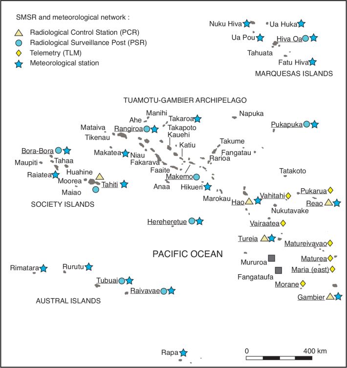Ministère de la Défense, 2006).

The SMSR network included Radiological Control Stations (PCR, Postes de Contrôle Radiologique), Radiological Surveillance Posts (PSR, Postes de Surveillance Radiologique), and Telemetry Measurements stations (TLM). PCRs and PSRs were responsible for the measurements of exposure rate in air, total beta-concentration in air and deposition density on the ground surface, a substantial difference between the two types of stations being that the PCRs were manned by radiation protection technicians, whereas the PSRs could be operated by non-specialized personnel. The TLM stations, in which measurements of exposure rate were conducted, were located on small low-populated and uninhabited islands and atolls in the southeastern part of Polynesia close to the test sites of Mururoa and Fangataufa. All results of the SMSR network were relevant to the purposes of reconstruction of ground deposition of radionuclides. Figure 4 shows the locations of PCRs, PSRs and TLMs in French Polynesia during the time period of the atmospheric nuclear tests. It should be noted that the numbers of PCR and PSR varied from year to year. In addition, measurements of total beta- concentration in air were performed in 1966 in Moorea, Raiatea (Society Islands) and in Anaa, Makemo, Hikueri, Takaroa (Tuamotu); however, these locations were not included in the SMSR network in later years and are not shown on Figure 4. In addition to the SMSR reports, meteorological information, namely daily precipitation and wind speed and direction, was available from Météo France; the location of the 23 meteorological stations is also shown on Figure 4.

The SMCB network was responsible for the measurements of radioactivity in biological samples, i.e. fresh cow’s milk produced on Tahiti, other foodstuffs, plants, lagoon and ocean fish, mollusks, etc. Only results of measurements of ¹³¹I in fresh cow’s milk from SMCB reports (SMCB, 1970, 1972, 1973) were considered.

More results of measurements were available in the declassified SMSR (SMSR, 1966-1975) reports in comparison with those available in UNSCEAR reports: 7,526 vs 439 for total beta-concentration in filtered air, 251 vs 0 for ground deposition density, 339 vs 2 for exposure rate, respectively. The numbers of measurements of ¹³¹I activity concentration in cow’s milk were found to be similar in the SMCB reports (SMCB, 1970, 1972, 1973) and in the reports to UNSCEAR.

Figure 4 Locations of SMSR network (underlined names of islands and atolls) and meteorological stations in French Polynesia in 1966-1974 (Drozdovitch et al., 2020a)

Figure 4

Figure 4 Locations of SMSR network (underlined names of islands and atolls) and meteorological stations in French Polynesia in 1966-1974 (Drozdovitch et al., 2020a)

Estimation of the time of arrival of fallout (TOA)

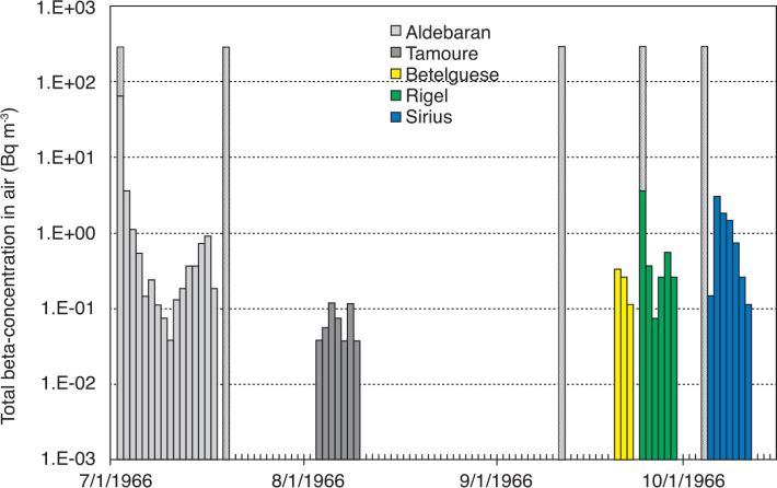
For the tests conducted in French Polynesia and for the 49 islands and atolls of interest, the values of TOA were preferably taken from the SMSR reports (SMSR, 1966-1975), the reports to UNSCEAR (Republic of France, 1967, 1969, 1971-1975), or the report from the Ministère de la Défense (2006). When the TOA values were not available in those reports, they were estimated from the results of measurements of daily total beta-concentration in air. Because of the horizontal and vertical wind shear, the radioactive clouds produced by the nuclear weapons tests usually followed different trajectories during the atmospheric transport over the large territory of French Polynesia; and there were many cases where “secondary fallout” extended over several days and where there were not one, but several waves of ground deposition. Figure 5 shows, for example, the variation with time of the daily total beta-concentration in air measured in Gambier Islands after the tests conducted in 1966: one part of the radioactive cloud from test Aldébaran (conducted on 2 July 1966) led according to data from SMSR (1966a) to direct fallout that reached Gambier at TOA = H+10h45 (“H” denotes time of detonation). Secondary fallout after test Aldébaran started at Gambier at H+9 d, and maximal concentration of total beta-concentration in air was reached on days 13 and 14 after the test. TOA for secondary fallout was taken to occur during the time of maximal concentration and to be H+13 d. The same considerations were applied for TOA after test Rigel (conducted on 24 September 1966): TOA for direct fallout was taken as H+12 h according to SMSR (1966b) and TOA of H+4 d for secondary fallout was derived from the temporal variation of the results of measurements of daily total beta-concentration in air (Figure 5).

Estimation of the ground deposition density

Figure 5 Variation with time of daily total beta-concentration in air measured in Gambier Islands after the tests conducted in 1966. Bar with pattern fill shows date of the test (Drozdovitch et al., 2020a)

Figure 5

Figure 5 Variation with time of daily total beta-concentration in air measured in Gambier Islands after the tests conducted in 1966. Bar with pattern fill shows date of the test (Drozdovitch et al., 2020a)

With a few exceptions, measurements of radionuclide composition in air or in fallout were not available to us for the atmospheric tests conducted in French Polynesia. To estimate the activities of specific radionuclides deposited on the ground, the results obtained for the atmospheric nuclear weapons tests conducted in the 1950s at the Nevada Test Site (NTS) in the USA were used. For these tests, Hicks (1981) calculated the deposition densities of radionuclides, normalized to an exposure rate of 1 mR h^-1 at 12 hours post-detonation (H+12h), for different types and platforms of nuclear weapons tests and for different times of arrival of fallout (TOA). Hicks (1981) data indicate that although the variability of the normalized deposition density for specific radionuclides from test to test may be substantial, there is little difference in the total deposition densities. Using data from 33 representative tests conducted at the NTS, deposition densities were calculated for fractionation values (ratios of refractory and of volatile radionuclides, R/V) equal to 0.5 (15 tests) for tower tests and equal to 1.0 (18 tests) for balloon tests. Use of the mixture of R/V values reflects conditions at French Polynesia where direct fallout occurred in islands close to the test sites (R/V = 1.0) as well as secondary fallout in distant locations with TOA up to H+20 d (R/V = 0.5). Table 7 shows the medians of the normalized total deposition densities and deposition densities of important radionuclides at different TOAs derived from reports of Hicks (1981). These tabulated values were used to reconstruct fallout from tests conducted in French Polynesia.

Tableau 7 Calculated median deposition densities of selected radionuclides at different TOAs normalized to an exposure rate of 1 mR h^-1 at 12 hours post-detonation (H+12h) (estimated from Hicks, 1981)

^a ICRP (2008).
^b (Eckerman and Ryman, 1993).

For some tests, measurements of total deposition density on the ground surface from direct fallout were available for some atolls and islands. In such instances, the deposition density of a given radionuclide was estimated by normalizing the total deposition density at TOA (Hicks, 1981) to the measured total deposition. If measurement of total deposition on the ground surface was not available, the following approaches were used to determine the deposition densities of the various radionuclides, depending on the type of data available for the locations of interest.

• Approach #1. An exposure-rate measurement was available

Step 1. The measured exposure rate was corrected to time H+12h using the assumption that the exposure rate varied with time after detonation, t in hours, according to t^-1.2 during the first week after the test (Dunning 1958).

Step 2. The deposition density of a particular radionuclide was estimated by multiplication of the corrected exposure rate (obtained in step 1) by the normalized deposition density at TOA calculated by Hicks (1981).

• Approach #2. Measurements of ¹³¹I concentration in milk
were available:

Step 2. The deposition density of any radionuclide other than ¹³¹I was estimated using the ratio of ¹³¹I deposition density at TOA (Hicks, 1981) to that obtained in step 1 as a scale.

• Approach #3. A measurement of total beta-activity in filtered air
was available:

Step 2. The deposition density of a particular radionuclide was estimated by normalizing the total deposition density at TOA (Hicks, 1981) to that obtained in step 1.

When radiation measurements were not available for the considered islands or atolls, the deposition densities of the various radionuclides were estimated from values of total beta-activity in filtered air obtained for given island or atoll by interpolation on distance between or from nearest location with available measurements (see Drozdovitch et al. (2020a) for detail).

As a result, ground deposition densities of 33 radionuclides were reconstructed for each of the 41 atmospheric tests in the 49 islands and atolls in French Polynesia where the study subjects resided during the atmospheric test period. Table 8 shows the total and the ¹³¹I deposition densities estimated for these 49 islands and atolls and indicate the test that contributed the most to the fallout that occurred in each location. The tests that contributed the most to the radioactive fallout in each archipelago of French Polynesia were:

Table 9 gives examples of radiation data available for Tahiti and of reconstructed deposition densities. As mentioned above, test Centaure (17/07/1974) resulted in the highest radioactive contamination of the most populated island in French Polynesia. Tests Sirius (4/10/1966) and Arcturus (2/07/1967) also resulted in substantial deposition in Tahiti. All other tests contributed less than 6% to the total deposition from all tests. Regarding ¹³¹I, tests Centaure, Sirius and Arcturus contributed around 85% of the ¹³¹I deposition in Tahiti.

For several tests and locations, the deposition densities obtained in this study using different approaches could be compared with the deposition densities reported by SMSR and Bourges (1997) (Table 10). The ratios of the deposition densities estimated in this study by different approaches to the deposition densities reported by SMSR and Bourges (1997) are characterized by an arithmetic mean ± standard deviation of 0.9±0.4, a geometric mean of 0.8 and range from 0.2 to 1.5 for approach #1 (13 deposition events); the corresponding values for approach #2 (8 deposition events) are 1.2±1.2 for the arithmetic mean, 0.9 for the geometric mean, and 0.4-4.0 for the range; for approach #3 (3 deposition events), the obtained values are 0.6±0.4 for the arithmetic mean, 0.6 for the geometric mean, and 0.4-1.1 for the range. For most deposition events (19 from 24, 79.2% of the total) a good agreement (within a factor of 2) was observed between the deposition densities estimated in this study and those reported in the literature.

A detailed description of the results of the study on reconstruction of ground deposition of radionuclides in French Polynesia resulting from atmospheric nuclear weapons tests at Mururoa and Fangataufa atolls can be found in Drozdovitch et al. (2020a).

Tableau 8 Total and ¹³¹I deposition densities from atmospheric nuclear weapons tests conducted in French Polynesia for the 49 islands and atolls where the study subjects resided in 1966-1974 (Drozdovitch et al., 2020a)

^a Direct fallout / secondary fallout.

Tableau 9 Reconstructed deposition densities on Tahiti island from the atmospheric nuclear weapons tests conducted in French Polynesia (Drozdovitch et al., 2020a)

^a Direct / secondary fallout.
^b Using approach #3.
^c Reconstructed using measured total deposition.

Tableau 10 Deposition densities at TOA reconstructed in this study using different approaches and measured (Bourges, 1997; SMSR, 1966b, 1967b, 1968-1969, 1970c, 1971a, 1973b, 1974a, b, 1975)

^a Declassified report of Joint Radiological Safety Service (SMSR, 1966b, 1967b, 1968-1969, 1970c, 1971a, 1973b, 1974a, b, 1975), unless otherwise indicated.
^b Bourges (1997).
^c Measured deposition density is given for Mahina.

Thyroid doses to French Polynesians resulting from atmospheric nuclear weapons tests: estimates based on radiation measurements
and population lifestyle data

Essentially the same methodology was used to calculate thyroid doses in TD08 (Drozdovitch et al., 2008) and TD19 (Drozdovitch et al., 2020b). As it was indicated above, new radiation measurements available from declassified reports and population lifestyle and consumption data collected during the focus group study were used in TD19.

Assessment of the internal doses resulting from inhalation

Figure

where V_k^air is the age-dependent breathing rate of the study subject (m³ s^-1) (ICRP 2002); RF^air is the reduction factor associated with indoor occupancy (unitless). As buildings in French Polynesia are very open for outdoor air circulation, RF^air = 1 was applied in the calculations; TIA_i^air is the time-integrated concentration of radionuclide i in air (Bq s m^-3); DC_i,k^inh is the age-dependent inhalation dose coefficient for the thyroid, i.e. the thyroid dose due to inhalation of unit activity of radionuclide i by a study subject of age k (mGy Bq^-1) (ICRP, 1995).

Values of total time-integrated concentration in air were taken from SMSR reports or estimated as described by Drozdovitch et al. (2020a). The value of the time-integrated concentration in air of specific radionuclide i was derived from the radionuclide mix at time of arrival of fallout (TOA) calculated by Hicks (1981) assuming that the radionuclide composition in filtered air was the same as that in the activity deposited on the ground. If the total deposition density was measured, an estimate of the time-integrated concentration of radionuclide i in air was obtained from the deposition density and the effective deposition velocity of radionuclide onto the ground surface:

where σ_i is the deposition density of radionuclide i at TOA (Bq m^-2); n = 1.76 × 10^-2 or 6.2 × 10^-2 m s^-1 is the effective deposition velocity of radionuclides onto the ground surface in case of dry deposition or of light rain (R < 1 mm d^-1) (UNSCEAR, 1993) or wet deposition (Drozdovitch et al., 2008), respectively. The assumption was made that the radionuclide distribution in the deposited activity was not influenced by the type of deposition, i.e. wet vs dry.

Thyroid dose due to ingestion of radioiodine isotopes and ¹³²Te

Figure

where DC_i,k^ing is the age-dependent ingestion dose coefficient for the thyroid, i.e. the age-dependent internal thyroid dose due to intake via ingestion of unit activity of radionuclide i by a study subject of age k (mGy Bq^-1) (ICRP, 1993, 1996a); V_m,k is the consumption rate of foodstuff m and drinking water by the subject of age k (kg (L) d^-1); PF_i,m is the processing factor, i.e., the fraction of radionuclide i remaining in foodstuff m after washing, culinary preparation and time delay between production and consumption (unitless); TIA_i,m^food is the time-integrated concentration of radionuclide i in foodstuff or drinking water m (Bq d kg^-1 (L^-1)).

• Estimation of consumption rates at age k from the consumption rates reported for age 15

where V_m,k is the consumption rate of foodstuff m by a study subject at age k (kg (L) d^-1); V_m,15 is the consumption rate of foodstuff m at age 15 that was reported by the study subject during her or his personal interview (kg (L) d^-1); SF_m,k is the scaling factor to adjust the consumption rate of foodstuff m at age 15 to that at age k (unitless). Table 11 shows, as example, values of the scaling factor, SF_m,k, that were derived for Tahiti and Tuamotu archipelago (except Gambier Islands) from a focus-group survey of dietary patterns in French Polynesia (Drozdovitch et al., 2020b).

Tableau 11 Scaling factors, SF_m,k, for age-dependent consumption rates of foodstuffs for Tahiti and Tuamotu archipelago (except Gambier Islands) (Drozdovitch et al., 2020b)

^a Did not consume this foodstuff at this age.
^b Including pota, watercress, spinach, lettuce.
^c Leaves of taro.
^d Did consume this foodstuff, but it was not locally produced.
^e Either from sea or from lagoon.

• Estimation of the time-integrated concentration in local cow’s milk
in Tahiti

The time-integrated concentration of radionuclide i in fresh cow’s milk locally produced in Tahiti, TIA_i,milk, was obtained as the integral over time from TOA to infinity of the concentration at time t (Müller and Pröhl, 1993; NCI, 1997):

Figure

where A_i,milk(t) is the concentration of radionuclide i in milk at time t (Bq L^-1); F*_i is the mass-interception coefficient of radionuclide i by grass, i.e. the fraction of radionuclide initially retained by unit mass of grass or of leafy vegetable: 0.7 m² kg^-1 (fresh weight) for iodine and tellurium for dry deposition, and 0.1 m² kg^-1 for iodine and 0.2 m² kg^-1 for tellurium for wet deposition (Gavrilin et al., 2004); I_g = 40 kg d^-1 is the daily intake of grass by cows, fresh weight; TF_i is the cow’s intake-to-milk transfer coefficient of radionuclide i (d L^-1). It was taken to be 3×10^-3 and 5×10^-4 d L^-1 for stable iodine and tellurium, respectively (Müller and Pröhl, 1993); λ^m_i is biological transfer rate in cow’s milk: 0.99 and 0.69 d^-1 for stable iodine and tellurium, respectively (Müller and Pröhl, 1993); λ^w_i is the elimination rate of radionuclide i from grass due to processes of weathering and growth dilution: 0.069 and 0.047 d^-1 for stable iodine and tellurium, respectively (Miller and Hoffman, 1983; Müller and Pröhl, 1993); λ^r_i is the radioactive decay constant of radionuclide i (d^-1).

The measured concentration of ¹³¹I in milk produced in Tahiti after the test Centaure (Republic of France, 1975) provided the opportunity to validate the ¹³¹I concentration obtained using this method. The measured (Republic of France, 1975) and the calculated ¹³¹I concentration in cow’s milk are compared in Figure 6. There is good agreement between the two sets of values.

Figure 6 131I activity in cow’s milk produced in Tahiti after the test Centaure: calculation (curve) and measurements (open circles) (Drozdovitch et al., 2008)

Figure 6

Figure 6 131I activity in cow’s milk produced in Tahiti after the test Centaure: calculation (curve) and measurements (open circles) (Drozdovitch et al., 2008)

• Estimation of the time-integrated concentration in leafy vegetables

To calculate the thyroid dose arising from ingestion of radionuclides with leafy vegetables using eqn. (3), the values of the processing factors, PF_i,LV, for radioiodine isotopes were taken to be equal to 0.5 for watercress (washing) and 0.7 for fâfâ, pota and spinach (washing and boiling) (IAEA, 1997). For ¹³²Te, the values of the processing factors were taken to be equal to 1.0 for watercress (washing) and 0.9 for fâfâ, pota and spinach (washing and boiling).

Results of measurements of total gamma-activity in leafy vegetables were available only as averages during a trimester (Republic of France, 1967, 1969, 1971-1975). Figure 7 compares the total gamma concentrations in leafy vegetables measured in Tahiti after test Centaure and calculated using this method. In general, the model provides estimates that are in reasonable agreement with the measurements.

• Estimation of the time-integrated concentration in drinking water

Figure

where A_i,water(t) is the water concentration of radionuclide i in the cistern at time t (Bq L^-1); W(t) is the amount of water in the cistern at time t (L); A_i,water(t – 1) is the water concentration of radionuclide i in the cistern at time t-1 day (Bq L^-1); W(t – 1) is the amount of water in the cistern at time t-1 day (L); Δt = 1 d is the calculation step; W_cons is the amount of cistern water consumed daily (L); S_coll is the area of rainwater collection for the cistern (m²); SL is the solubility of radioisotopes in rainwater (unitless). The solubility of radioiodine isotopes and ¹³²Te in rainwater was taken to be 0.2 (Lessard et al., 1973) for direct fallout with TOA of H+24h or less. For TOA greater than one day, the solubility of radioiodine isotopes was taken to be equal to 1.

Figure 7 Total gamma-activity in leafy vegetables in Tahiti after the test Centaure: calculation (curve) and average measurements during a trimester in lettuce (thin line) and fâfâ (broken line) (Drozdovitch et al., 2008)

Figure 7

Figure 7 Total gamma-activity in leafy vegetables in Tahiti after the test Centaure: calculation (curve) and average measurements during a trimester in lettuce (thin line) and fâfâ (broken line) (Drozdovitch et al., 2008)

Figure

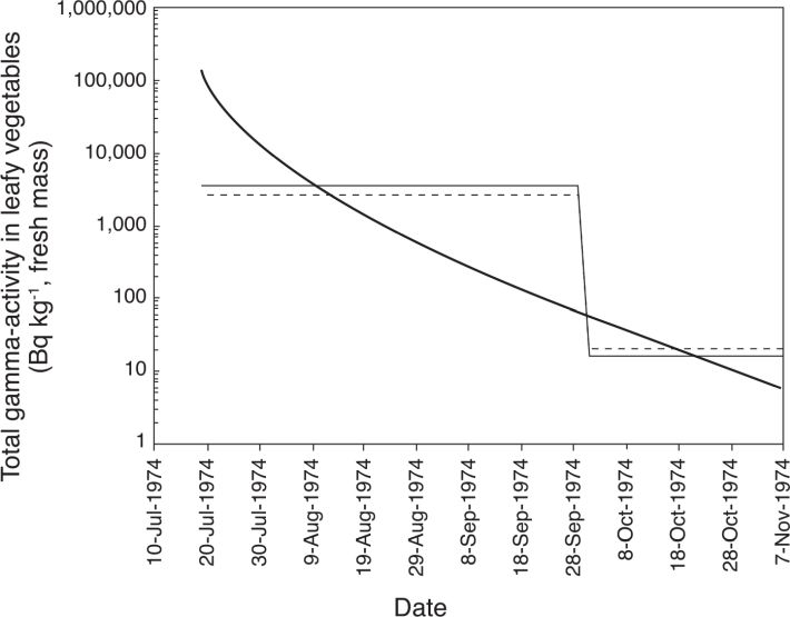
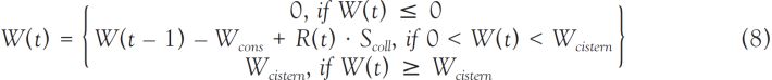where R(t) is the precipitation on day t (Météo France, 2005) (mm); W_cistern is the volume of the cistern equals to 15,000 and 90,000 L for family and communal cisterns, respectively (HCRFP, 1977).

Figure

The daily consumptions of water from the cistern were 200 and 2000 L for family and communal cisterns, respectively, and the areas of rainwater collection for the cisterns were 30 and 200 m², respectively (Drozdovitch et al., 2019). The amount of water in the cisterns was calculated for each year of atmospheric testing for the time period starting 2 weeks before the first nuclear weapons test and ending 5 weeks after the last test of the year. The initial content of rainwater in the cistern was assumed to be 1/4 of its volume. The model considers that the daily consumption of drinking water varied from 0.25 L for 0-12 mo to 2.0 L for adults.

Thyroid dose due to external irradiation from radionuclides deposited
on the ground

Figure

where BF_k is the behavioral factor that takes into account the fraction of time spent indoors by the subject of age k and the shielding properties of residential building (unitless); DC_i,k^ext is the thyroid dose rate coefficient for radionuclide i, that is, the absorbed dose rate in the thyroid (mGy d^-1) per unit deposition (Bq m^-2) of radionuclide i in a plane source covered by 3 mm of soil representing ground roughness (Bellamy et al., 2019); t₁ and t₂ are the times of beginning and end of residence at a given location (d).

Figure

where SF is the shielding factor, which is related to the attenuation of the gamma rays emitted outdoors by the building material of the dwellings (unitless). It was 0.1 for concrete, 0.3 for wood and 0.7 for straw and bamboo (Drozdovitch et al., 2008); T_indoors,k is the time spent indoors in a day by a subject of age k, which depends for schoolchildren aged 7-14.9 y on the time of year: school days or school vacation (from 15 June to 15 August) (h). Age-, archipelago- and season-specific values of time spent indoors for the Polynesian population was collected by Drozdovitch et al. (2019); LF is the location factor for outdoor conditions that depends on the type of environment (unitless). It was taken to be 0.5 for a typical urban environment and 0.7 for a rural environment (Drozdovitch et al., 2008).

Table 12 provides the values for BF_k, calculated using eqn (11), that were used in this study. If the study subject reported during the personal interview the type and construction material of residence, the value of the behavioral factor corresponding to age k of the study subject and to her/his archipelago and type of residence was used in the dose calculation. If the study subject did not recall the type and construction material for her/his residence, the behavioral factor was estimated using the archipelago-specific distribution of types and construction materials of residences that were reported by the focus groups to be typical in the 1960s-1970s (Drozdovitch et al., 2019).

Ingestion of long-lived ¹³⁷Cs with foodstuffs

Figure

where N is the number of days of residence in a given archipelago during which the contaminated foodstuffs were consumed (d) in the year under consideration; D_k^Cs is the age-dependent thyroid dose coefficient for ¹³⁷Cs ingestion (ICRP, 1993) (mGy Bq^-1); V_m,k is the consumption rate of foodstuff m by the subject of age k (see Table 2 for the list of foodstuffs) (kg (L) d^-1); PF_m^Cs is the processing factor that reflects the change in activity concentration of ¹³⁷Cs resulting from the culinary preparation of the raw product (unitless); A_m^Cs is the average annual concentration of ¹³⁷Cs in foodstuff m for each year from 1966 to 1974 (Bq kg^-1(L^-1)).

Archipelago-specific average annual concentrations of ¹³⁷Cs in foodstuffs were derived from the results of measurements of ¹³⁷Cs in foodstuffs provided in reports to UNSCEAR (Republic of France, 1967, 1969, 1971-1975) and in de-classified reports (SMSR, 1970; SMCB, 1975a,b, 1976a,b, 1978a,b).

Tableau 12 Archipelago-specific values of the behavioral factor, BF_k (Drozdovitch et al., 2020b)

^a Only in Raiatea.
^b For unknown type of residence, behavior factor was estimated using archipelago-specific combination of type and construction material of residences according to Drozdovitch et al. (2019).
^c During school days.
^d During school vacation from 15 June to 15 August.

To calculate the thyroid dose arising from ingestion of ¹³⁷Cs using eqn. (12), the values of the processing factor were equal to 0.6 for root vegetables, 0.7 for fâfâ and pota, 0.8 for meat, 0.9 for leafy vegetables (except fâfâ and pota), fish, and uru (IAEA, 1997). For foodstuffs other than those listed above, the value of the processing factor was 1.0.

Study subjects exposed in utero

Figure

where V^air_adult is the breathing rate of the mother of the study subject (m³ s^-1) (ICRP, 2002); DC^inh,i_fetus(t_g) is the thyroid dose coefficient to a fetus of gestational age t_g at time TOA of the test under consideration, per unit of acute inhalation intake of radioiodine or tellurium isotopes by the mother (ICRP, 2001) (mGy Bq^-1).

Figure

Archipelago-specific values of consumers’ fractions and of consumption rates of locally-produced foodstuffs by pregnant women, which were obtained during the focus-group study (Drozdovitch et al., 2019), are given in Table 13. The consumption rate of foodstuff m by pregnant women used in this study, V*_m,preg, was calculated from the focus-group data as:

Breastfed study subjects

Tableau 13 Archipelago-specific fractions of consumers (_Pcons,preg) and consumption rates^a of locally produced foodstuffs, V_m,preg (kg (L) d^-1), by pregnant women (Drozdovitch et al., 2020b)

^a Consumption rates are provided for consumers only.
^b Leafy vegetables including pota, watercress, spinach, lettuce.
^c Foodstuff consumed but not locally produced.

Figure

where DC^inh,i_brfed is the thyroid dose coefficient to a breastfed child due to inhalation of a specific radioiodine or tellurium isotope by the mother (ICRP, 2004) (mGy Bq^-1).

Figure